For any queries, email us at [email protected]


For any queries, email us at [email protected]


For any queries, email us at
[email protected]
")

The motivation behind this article is to explore pair-trading opportunities between cryptocurrencies. Pairs trading is well explored in equities and other asset classes and enough literature is available on it. We’ve applied some of those techniques to cryptocurrencies and are sharing our findings here.
There are many ways of trading pairs but in this article we only touch upon statistical arbitrage for identifying long-short pairs.
Statistical arbitrage involves entering a long-short trade on two assets such that the resulting portfolio is hedged, i.e. the net gain from owning this portfolio, should be zero. The idea here is to stay risk neutral and to profit from the relative movement between two coins. In stat-arb, we identify hedged portfolios which have diverged from their mean (i.e. starting to yield non-zero returns) and bet on their convergence.
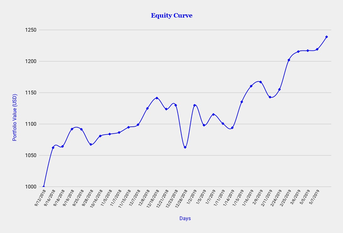
Below are the results from trading BTC-ETH statistical arbitrage long-short pair between Sep’18 and May’19.
| Stat-Arb Pair | BTC-ETH |
|---|---|
| Duration | Sep’18 – May’19 |
| Portfolio Return (Unlevered) | 23.90% |
| Max Drawdown | -7.80% |
| Total Trades | 30 |
| Winning Trades | 22 |
| Win Percentage | 73.33% |
| Average Trade Duration (days) | 1.26 |
| Index Equity Value | 1000$ |
| Index Final Value | 1239$ |
We observed 30 incidences of divergence over over this time. 22 of these incidences have shown expected convergence and have resulted in profits.
Equity curve is plotted assuming we start with 1000$ at beginning of the strategy and further invest only 1000$ in the next trade, i.e. profits are not reinvested. The strategy is supposed to stay risk neutral hence the best benchmark to compare the strategy return is risk-free interest rate and not BTC or ETH return.
What's in this post
As the name suggests statistical arbitrage is an arbitrage but unlike other arbitrages, stat-arb. is not-risk-free. It’s more like a statistical truth which is observed. Of-course statistical truths can break in light of certain events or fresh data and this needs to be accounted for in real trading.
In order to select cryptos for stat-arb we look for crypto-assets that show strong co-movement. In statistics we use correlation to measure co-movement. However, for building a hedged portfolio we look for co-integration and not correlation.
Two data sets are said to be correlated if change in one can be explained by change in another (this is not causation, just observed co-movement). Higher the correlation higher the degree of co-movement. However, correlation alone might not necessarily result in profitable long-short pairs trading. High correlation while necessary is not a sufficient condition for selecting a long-short trading pair. Let’s see why?
Assume that there are two coins: A and B, which exhibit high correlation in daily returns. This would imply that when A moves up, B also moves up. The amount by which B is expected to move up can be calculated using regression between returns of Coin A and Coin B. Let’s say that the regression co-efficient of A and B is 0.6. Thus for a 5% move-up in price of coin A we’d expect a 3% move-up in the price of coin B.
Assume that Coin A moves-up 5% for 10 consecutive days. We’d expect Coin B to move 3% for each of these days. This would mean that the price series for both these coins will start to diverge as in Exhibit1.
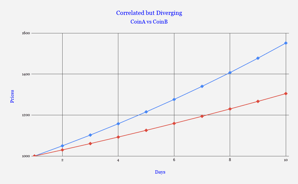
It is difficult to profit from such situations because buying/selling any asset naked would mean assuming directional risk in that asset. Which goes against our premiss of entering a long-short risk neutral portfolio to avoid taking any directional risk.
In the above example buying Coin B would result in profits but in real life, assets will not move unidirectionally and it’s almost impossible to comment on the next move. Hence we look for a solution where we can profit from the relationship between these two assets without assuming directional risk in any of them.
This is where co-integration is comes into picture. Two times series (returns against time for our discussion) are called co-integrated if we can find some linear combination of them to remain stationary with time (in simple but slightly inaccurate words not moving with time). Thus 2 coins are co-integrated, if we can find a portfolio (some quantity of Coin A and some quantity of Coin B) such that this portfolio stays around a constant value over time.
This is interesting because offsetting positions in these two coins will cancel out any market risks (β) and what will be left is pure-play catch-up/co-movement trade.
Referring to the previous example, consider a portfolio which is Long 1 units of A and Short 1.6 unit of B, the return of that portfolio can be given as:
Rp = Ra – 1.6*Rb
We’d always expect the return of this portfolio to be zero over a period of time. Anytime the return of the portfolio diverges away from zero, we have a trade.
Two time-series At and Bt are called co-integrated if there exists some linear combination of these series, which is a stationary time-series. Hence, if we can find some value of lambda (λ) such that
Ct = At – λ*Bt ,
is a stationary time series, then At and Bt are called co-integrated.
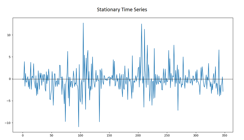
A time series is called stationary if it’s mean and variance stay constant over time and if its covariance with itself, over any interval, remains constant. The stationarity of a time series makes it predictable. Constant mean makes the series converge towards the mean should it diverge away from the mean and vice-versa.
How does a stationary time-series looks like?
Should two time series exhibit strong correlation, it is compelling to test them for co-integration. In finance, this is of importance because this would mean we can find a portfolio, using these 2 assets, which has a degree of predictability in its returns.
Lets say At represents the returns of the first coin and Bt represents the returns of second coin. If we can find a λ, which makes Ct stationary, then we have discovered a portfolio whose returns will be mean-reverting.
Note that a cash-future hedge portfolio will always be co-integrated. For example if At is Bitcoin Spot and Bt is Bitcoin Futures then for λ = 1, we have a hedged portfolio which will converge towards its mean. In other words premium and discounts on futures will eventually converge to fair-value of futures.
Hence λ is often referred to as hedge ratio.
There are lot of tests for checking co-integration but the most widely used is the ADF (Augmented Dickey Fuller test). It starts with a null hypothesis that there is no co-integration or that the co-integrated series has a unit-root. If we are able to reject the null hypothesis we can expect co-integration.
Hence we first spot correlation in returns, calculate the regression co-efficient. Prepare a hedge portfolio and test it for co-integration.
Steps of building the strategy and identifying trade:
We are going to start with testing correlation of BTC and ETH. We have used daily candles/intervals for our data. We form a training data-set and a test data-set and backtest our strategy.
The daily price correlation of BTC & ETH : 0.81
Regression coefficient between BTC and ETH: 0.64
We are now going to test the spread series,
st = rBTC – λ * rETH ,
for stationarity using the ADF test (Advanced Dickey Fuller test). The test is available as a straight-up utility in Matlab, R and Python. We have used Python for our analysis.
We found that the p-value from the ADF test is low enough to reject the null hypothesis. Hence we can safely assert that our spread portfolio is indeed stationary. You can reject the null hypothesis when the p-value is less than or equal to 0.05 or 5%.
Further we check our spread for normality and find it to be normally distributed.
Once we have established co-integration in returns of BTC & ETH, the next step is to build a trading strategy to profit from statistical arbitrage. As a part of this strategy we are going to monitor the return of the co-integrated portfolio.
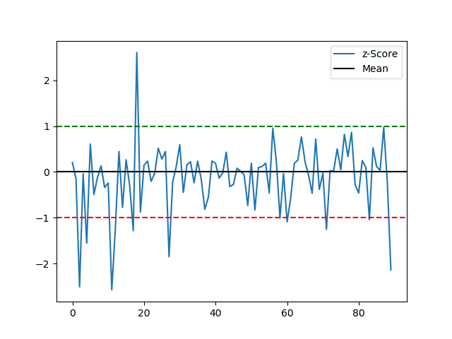
When the portfolio moves certain standard deviations below mean, we will enter into a long position on the portfolio and when it moves certain SDs above mean we shall assume a short position in the portfolio.
We have represented every point on the spread series in terms of z-score, i.e. how many standard deviations, is that point away from the mean?
zi = (xi – μ) / 𝜎
Where xi = Value of spread series at any point, μ = Mean of the series, 𝜎 = Standard Deviation of the spread series.
Using our training data we find λ, μ and 𝜎. We assume that these values stay constant for test-data on which we are going to run our backtesting. Further we compute the backtested results of our long-short statistical arbitrage strategy applied over BTC & ETH.
We have backtested the strategy over data from spot market. We have used prices of BTC-USDT and ETH-USDT pairs for backtesting.
In order to execute this strategy in live trading, we recommend using futures contracts. The futures contracts used should be USD quoted for both BTC and ETH. You can use BTCUSD June futures and ETHUSDQ June futures on Delta Exchange to trade this strategy.
ETHUSDQ futures are quoted in USD and settled in USDC hence they mimic true exposure of ETH to USD, which makes them best choice for executing these trades.
| Stat-Arb Pair | BTC-ETH |
|---|---|
| Duration | Sep’18 – May’19 |
| Portfolio Return (Unlevered) | 23.90% |
| Max Drawdown | -7.80% |
| Initial Equity | 1000$ |
| Final Equity | 1239$ |
| Total Trades | 30 |
| Winning Trades | 22 |
| Avg. Return Winning Trades | 1.93% |
| Losing Trades | 8 |
| Avg. Return Losing Trades | -2.32% |
| Total Profits | 424.75$ |
| Total Losses | -185.73$ |
| Avg. Duration Winning Trades (days) | 1.18 days |
| Avg. Duration Losing Trades (days) | 1.46 days |
The execution cost of the trade in futures will not be more than 65bps un-levered for round-trip (entry and exit). The returns we have demonstrated above are un-levered 2-way returns. Executing on futures will further increase the return multifold due to leverage.
With a 10x leverage, per trade return will grow to 7.97% which reduces to 7.3% post execution costs. Assuming 30 bps slippage for entire trade we expect a 7% average trade return, when using leverage.
Instead of looking at a return based stop, we have used stop on our spread series. Once the stop series moves 3.5 standard deviations away from the mean. We exit the trade.
We have also tried with time based stop-losses but have found that spread based stops perform best.
You can also use absolute return based stop-loss but we have not used that.
The high correlation in prices of cryptocurrencies is the precursor for long short pairs trading. We find that a long-short risk neutral strategy ends up giving good returns. The key to success and improving the results is weeding out bad trades i.e. setting up right filters/stop-loss; in order to timely close loss making trades. We encourage readers to try with different training, testing periods, stop-loss strategies and share results.
We are going to implement this strategy over a few other cryptocurrencies and publish results in due course. We are also going to set-up a dashboard on our analytics page for users to monitor spread series for BTC-ETH and its recent history.
We would love your comments! Do let us know your thoughts on the results and strategy that we have published.
Should you like what we have shared, do reward us with your trades on Delta Exchange.
Stay Connected With News, Updates And More
